Probability

Probability is the branch of mathematics concerning numerical descriptions of how likely an event is to occur. The probability of an event is a number between 0 and 1, where, roughly speaking, 0 indicates impossibility of the event and 1 indicates certainty. The higher the probability of an event, the more likely it is that the event will occur.

Probability theory provide mathematical abstractions of non-deterministic or uncertain processes or measured quantities that may either be single occurrences or evolve over time in a random fashion. It formalises probability in terms of a probability space, which assigns a measure taking values between 0 and 1, termed the probability measure, to a set of outcomes called the sample space. Any specified subset of these outcomes is called an event. Central subjects in probability theory include discrete and continuous random variables, probability distributions, and stochastic processes.

Axioms

• Random events are, by definition, unpredictable, but if the probability distribution is known, the frequency of different outcomes over repeated events (or trials) is predictable.
  A random (stochastic, aleatory) variable \( X \) is a variable whose values depend on outcomes of a random phenomenon.
• The sample (possibility) space \( \Omega \) is the set of all possible outcomes of a random phenomenon being observed. For example, the sample space of a coin flip would be {head, tail}.
• The event space \( F \) is a set of events, each event \( E \) being a subset of the sample space (effective out of the possible outcomes).
• A probability function \( P \) assigns to each event in the event space a probability, taking values between 0 and 1. It describes the probability \( P (X \in E) \) that the event \( E \), from the sample space, occurs.
• The probability function only characterizes a probability distribution if it satisfies all the Kolmogorov axioms :
  • \( P(X \in E) \geq O \space \space \forall E \in F \), probability is non-negative
  • \( P(X \in E) \leq 1 \space \space \forall E \in F \), no probability exceeds 1 | \( P(\Omega) = 1 \) , the probability that at least one of the elementary events in the entire sample space will occur is 1
  • \( P(X \in \bigsqcup_{i=1}^\infty E_{i}) = \sum_{i=1}^\infty P(X \in E_{i}) \) , the probability of the union of all events equals the sum of the probabilities of each event

Distributions

A probability distribution is a mathematical description of the probabilities of events, subsets of the sample space.

Discrete

The set of possible outcomes is discrete (countable). Probabilities are encoded by a discrete list of the probabilities of the outcomes, known as the Probability mass function (PMF) . It assigns a probability to each possible outcome and the probability of an event is then defined to be the sum of the probabilities of the outcomes that satisfy the event.

\( p_{X}(x_{i}) = P (X = x_{i}) \), the probability function \( p \) of random variable \( X \) for event outcome i equals the probability measure \( P \) of \( X \) being the outcome of the i^th event, whereby \( p_{X}(x_{i}) > 0 \) and \( p_{X}(x_{i}) > 0 \)
A classical example if the rolling of a die. The sample space for any number appearing on top is {1,2, ...,6}, for an even number appearing on top is {2,4,6}. The probability for any number is \( \frac{1}{6} \), for an even number is \( \frac{1}{3} \).

Continuous

When a random variable takes values from a continuum then typically, any individual outcome has probability zero and only events that include infinitely many outcomes, such as intervals, can have positive probability.

Probability density function	Cumulative distribution function
A Probability density function(PDF) describes the infinitesimal probability of any given value, and the probability that the outcome lies in a given interval can be computed by integrating the probability density function over that interval. A random variable \( X \) has a continuous probability distribution if there is a function \( f: \mathbb{R} \rightarrow [0,\infty] \) such that for each interval \( I \subset \mathbb{R} \), the probability of \( X \) belonging to \( I \) is given by the integral of \( f \) over \( I \). For example, if \( I=[a,b] \), then we would have: \( P[a \leq X \leq b] = \int_{a}^b \space f(x)dx\)	A Cumulative distribution function (CDF) , describes the probability that the random variable is no larger than a given value, corresponding to the area under the probability density function from \( -\infty \) to \( x \). \( F(x) = P[-\infty \leq X \leq x] = \int_{-\infty}^x \space f(x)dx\)

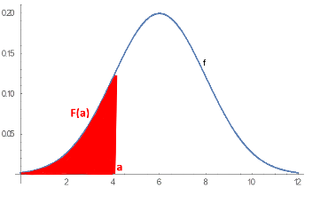
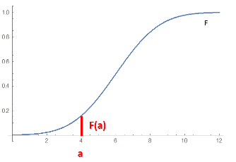
Normal distribution

There are multiple probability distributions identified, but the most widely adopted is the Normal (Gaussian) distribution , also known as the bell curve.

Be \( \mu \) the expected value (mean), \( \sigma \) the standard deviation of a normal distribution, the general form of its probability density function is : \( f(x) = N(\mu, \sigma^2) = \frac{1}{\sigma \space \sqrt{2 \pi}} e^{-\frac{1}{2} (\frac{\space x \space - \space \mu \space}{\sigma} )^2} \)

A normal distribution with a mean of 0 and a standard deviation of 1 is called Standard Normal distribution, described by this probability density function: \( f(x) = \frac{1}{\sqrt{2 \pi}} e^{-\frac{x^2}{2}} \)
The factor \( \frac{1}{\sqrt{2\pi}} \) ensures that the total area under the curve \( f(x) \) is equal to one. The factor \( \frac{1}{2} \) in the exponent ensures that the distribution has unit variance (i.e. equal to one), and therefore also unit standard deviation. This function is symmetric around \( x=0 \), where it attains its maximum value \( \frac{1}{\sqrt{2\pi}} \) and has inflection points at \( x = -1 \) and \( x = +1 \).

Normal distributions are used in mathematical finance to describe random fluctuations in asset prices for models that assume such prices are normally distributed.